Week 7

Agenda:

1. Automatic differentiation
2. Cross validation
3. Classification

Packages we will require this week

packages <- c(
    # Old packages
    "ISLR2",
    "dplyr",
    "tidyr",
    "readr",
    "purrr",
    "glmnet",
    "caret",
    "repr",
    # NEW
    "torch",
    "mlbench"
)

# renv::install(packages)
sapply(packages, require, character.only=TRUE)

---

Thu, Feb 23

In the last class we looked at the following numerical implementation of gradient descent in R

x <- cars$speed
y <- cars$dist

# define the loss function

Loss <- function(b, x, y){
    squares <- (y - b[1] - b[2] * x)^2
    return( mean(squares) )
}

b <- rnorm(2)
Loss(b, cars$speed, cars$dist)

[1] 1905.504

This is the numerical gradient function we looked at:

# define a function to compute the gradients

grad <- function(b, Loss, x, y, eps=1e-5){
    b0_up <- Loss( c(b[1] + eps, b[2]), x, y)
    b0_dn <- Loss( c(b[1] - eps, b[2]), x, y)
    
    b1_up <- Loss( c(b[1], b[2] + eps), x, y)
    b1_dn <- Loss( c(b[1], b[2] - eps), x, y)
    
    grad_b0_L <- (b0_up - b0_dn) / (2 * eps)
    grad_b1_L <- (b1_up - b1_dn) / (2 * eps)
    
    return( c(grad_b0_L, grad_b1_L) )
}

grad(b, Loss, cars$speed, cars$dist)

[1]   -73.13359 -1319.66565

The gradient descent implementation is below:

steps <- 9999
L_numeric <- rep(Inf, steps)
eta <- 1e-4
b_numeric <- rep(0.0, 2)

for (i in 1:steps){
    b_numeric <- b_numeric - eta * grad(b_numeric, Loss, cars$speed, cars$dist)
    L_numeric[i] <- Loss(b_numeric, cars$speed, cars$dist)
    if(i %in% c(1:10) || i %% 1000 == 0){
        cat(sprintf("Iteration: %s\t Loss value: %s\n", i, L_numeric[i]))
    }
}

Iteration: 1     Loss value: 2266.69206282174
Iteration: 2     Loss value: 2059.23910669384
Iteration: 3     Loss value: 1873.22918303142
Iteration: 4     Loss value: 1706.44585378992
Iteration: 5     Loss value: 1556.90178087535
Iteration: 6     Loss value: 1422.815045446
Iteration: 7     Loss value: 1302.58791495713
Iteration: 8     Loss value: 1194.78780492565
Iteration: 9     Loss value: 1098.13020855732
Iteration: 10    Loss value: 1011.46339084888
Iteration: 1000  Loss value: 258.373721118606
Iteration: 2000  Loss value: 257.10759589046
Iteration: 3000  Loss value: 255.892681655669
Iteration: 4000  Loss value: 254.726907082124
Iteration: 5000  Loss value: 253.608284616954
Iteration: 6000  Loss value: 252.534907097824
Iteration: 7000  Loss value: 251.504944501478
Iteration: 8000  Loss value: 250.516640823636
Iteration: 9000  Loss value: 249.568311085141

options(repr.plot.width=12, repr.plot.height=7)

par(mfrow=c(1, 2))

plot(x, y)
abline(b_numeric, col="red")

plot(L_numeric, type="l", col="dodgerblue")

---

Automatic differentiation

The cornerstone of modern machine learning and data-science is to be able to perform automatic differentiation, i.e., being able to compute the gradients for any function without the need to solve tedious calculus problems. For the more advanced parts of the course (e.g., neural networks), we will be using automatic differentiation libraries to perform gradient descent.

While there are several libraries for performing these tasks, we will be using the pyTorch library for this. The installation procedure can be found here

The basic steps are:

renv::install("torch")
library(torch)
torch::install_torch()

---

Example 1:

x <- torch_randn(c(5, 1), requires_grad=TRUE)
x

torch_tensor
-0.0658
 0.9932
 0.2550
 0.9097
-1.1083
[ CPUFloatType{5,1} ][ requires_grad = TRUE ]

f <- function(x){
    torch_norm(x)^10
}

y <- f(x)
y

torch_tensor
291.718
[ CPUFloatType{} ][ grad_fn = <PowBackward0> ]

y$backward()

\[ \frac{dy}{dx} \]

x$grad

torch_tensor
 -61.7160
 931.1658
 239.0168
 852.8220
-1039.0062
[ CPUFloatType{5,1} ]

(5 * torch_norm(x)^8) * (2 * x)

torch_tensor
 -61.7160
 931.1658
 239.0168
 852.8220
-1039.0062
[ CPUFloatType{5,1} ][ grad_fn = <MulBackward0> ]

---

Example 2:

x <- torch_randn(c(10, 1), requires_grad=T)
y <- torch_randn(c(10, 1), requires_grad=T)

c(x, y)

[[1]]
torch_tensor
 0.5419
-2.0761
-1.2139
-0.5452
-0.9114
 0.1124
 0.7301
 0.5995
-0.8506
 0.3153
[ CPUFloatType{10,1} ][ requires_grad = TRUE ]

[[2]]
torch_tensor
 0.2530
-1.1521
-0.7859
 0.9707
 0.3526
 0.7097
 0.2911
-0.9521
 0.7741
-0.7462
[ CPUFloatType{10,1} ][ requires_grad = TRUE ]

f <- function(x, y){
    sum(x * y)
}

z <- f(x, y)
z

torch_tensor
1.46023
[ CPUFloatType{} ][ grad_fn = <SumBackward0> ]

z$backward()

c(x$grad, y$grad)

[[1]]
torch_tensor
 0.2530
-1.1521
-0.7859
 0.9707
 0.3526
 0.7097
 0.2911
-0.9521
 0.7741
-0.7462
[ CPUFloatType{10,1} ]

[[2]]
torch_tensor
 0.5419
-2.0761
-1.2139
-0.5452
-0.9114
 0.1124
 0.7301
 0.5995
-0.8506
 0.3153
[ CPUFloatType{10,1} ]

c(x - y$grad, y - x$grad)

[[1]]
torch_tensor
 0
 0
 0
 0
 0
 0
 0
 0
 0
 0
[ CPUFloatType{10,1} ][ grad_fn = <SubBackward0> ]

[[2]]
torch_tensor
 0
 0
 0
 0
 0
 0
 0
 0
 0
 0
[ CPUFloatType{10,1} ][ grad_fn = <SubBackward0> ]

---

Example 3:

x <- torch_tensor(cars$speed, dtype = torch_float())
y <- torch_tensor(cars$dist, dtype = torch_float())

plot(x, y)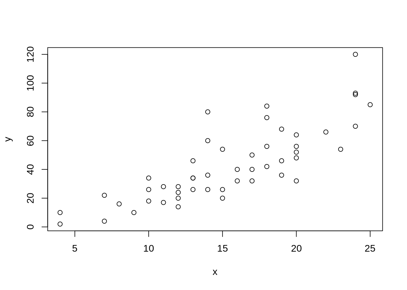

b <- torch_zeros(c(2,1), dtype=torch_float(), requires_grad = TRUE)
b

torch_tensor
 0
 0
[ CPUFloatType{2,1} ][ requires_grad = TRUE ]

loss <- nn_mse_loss()

b <- torch_zeros(c(2,1), dtype=torch_float(), requires_grad = TRUE) # Initializing variables
steps <- 10000 # Specifying the number of optimization steps
L <- rep(Inf, steps) # Keeping track of the loss


eta <- 0.5 # Specifying the learning rate and the optimizer
optimizer <- optim_adam(b, lr=eta)


# Gradient descent optimization over here
for (i in 1:steps){
    y_hat <- x * b[2] + b[1]
    l <- loss(y_hat, y)
    
    L[i] <- l$item()
    optimizer$zero_grad()
    l$backward()
    optimizer$step()
    
    if(i %in% c(1:10) || i %% 200 == 0){
        cat(sprintf("Iteration: %s\t Loss value: %s\n", i, L[i]))
    }
}

Iteration: 1     Loss value: 2498.06005859375
Iteration: 2     Loss value: 1759.53002929688
Iteration: 3     Loss value: 1174.45300292969
Iteration: 4     Loss value: 742.353759765625
Iteration: 5     Loss value: 457.703643798828
Iteration: 6     Loss value: 307.684936523438
Iteration: 7     Loss value: 270.263397216797
Iteration: 8     Loss value: 314.067993164062
Iteration: 9     Loss value: 401.761566162109
Iteration: 10    Loss value: 496.908325195312
Iteration: 200   Loss value: 231.474166870117
Iteration: 400   Loss value: 227.11474609375
Iteration: 600   Loss value: 227.070495605469
Iteration: 800   Loss value: 227.070404052734
Iteration: 1000  Loss value: 227.070404052734
Iteration: 1200  Loss value: 227.070404052734
Iteration: 1400  Loss value: 227.070404052734
Iteration: 1600  Loss value: 227.070404052734
Iteration: 1800  Loss value: 227.070404052734
Iteration: 2000  Loss value: 227.070404052734
Iteration: 2200  Loss value: 227.070404052734
Iteration: 2400  Loss value: 227.070434570312
Iteration: 2600  Loss value: 227.070434570312
Iteration: 2800  Loss value: 227.070434570312
Iteration: 3000  Loss value: 227.070434570312
Iteration: 3200  Loss value: 227.070434570312
Iteration: 3400  Loss value: 227.070388793945
Iteration: 3600  Loss value: 227.070404052734
Iteration: 3800  Loss value: 227.070434570312
Iteration: 4000  Loss value: 227.070404052734
Iteration: 4200  Loss value: 227.070434570312
Iteration: 4400  Loss value: 227.070434570312
Iteration: 4600  Loss value: 227.070434570312
Iteration: 4800  Loss value: 227.070404052734
Iteration: 5000  Loss value: 227.070404052734
Iteration: 5200  Loss value: 227.132614135742
Iteration: 5400  Loss value: 227.070434570312
Iteration: 5600  Loss value: 227.070404052734
Iteration: 5800  Loss value: 227.071762084961
Iteration: 6000  Loss value: 227.070434570312
Iteration: 6200  Loss value: 227.093811035156
Iteration: 6400  Loss value: 227.070434570312
Iteration: 6600  Loss value: 227.070434570312
Iteration: 6800  Loss value: 227.070877075195
Iteration: 7000  Loss value: 227.070404052734
Iteration: 7200  Loss value: 227.070617675781
Iteration: 7400  Loss value: 227.070404052734
Iteration: 7600  Loss value: 227.070404052734
Iteration: 7800  Loss value: 227.070404052734
Iteration: 8000  Loss value: 227.070404052734
Iteration: 8200  Loss value: 227.076507568359
Iteration: 8400  Loss value: 227.070434570312
Iteration: 8600  Loss value: 227.070434570312
Iteration: 8800  Loss value: 227.071090698242
Iteration: 9000  Loss value: 227.070434570312
Iteration: 9200  Loss value: 227.070434570312
Iteration: 9400  Loss value: 227.070404052734
Iteration: 9600  Loss value: 227.070434570312
Iteration: 9800  Loss value: 227.070434570312
Iteration: 10000     Loss value: 229.465744018555

options(repr.plot.width=12, repr.plot.height=7)

par(mfrow=c(1, 2))

plot(x, y)
abline(as_array(b), col="red")

plot(L, type="l", col="dodgerblue")

plot(L_numeric[1:100], type="l", col="red")
lines(L[1:100], col="blue")

Cross validation

df <- Boston %>% drop_na()
head(df)

     crim zn indus chas   nox    rm  age    dis rad tax ptratio lstat medv
1 0.00632 18  2.31    0 0.538 6.575 65.2 4.0900   1 296    15.3  4.98 24.0
2 0.02731  0  7.07    0 0.469 6.421 78.9 4.9671   2 242    17.8  9.14 21.6
3 0.02729  0  7.07    0 0.469 7.185 61.1 4.9671   2 242    17.8  4.03 34.7
4 0.03237  0  2.18    0 0.458 6.998 45.8 6.0622   3 222    18.7  2.94 33.4
5 0.06905  0  2.18    0 0.458 7.147 54.2 6.0622   3 222    18.7  5.33 36.2
6 0.02985  0  2.18    0 0.458 6.430 58.7 6.0622   3 222    18.7  5.21 28.7

dim(df)

[1] 506  13

Split the data into training (80%) and testing sets (20%)

k <- 5
fold <- sample(1:nrow(df), nrow(df)/2)
fold

  [1] 293 386 154 432 137 414 122 297 279 358 161 210 262  78 501 187  32 342
 [19] 352 356  29 257 441 268 368   6 497 367 458  84 176 185 301 332  30 377
 [37] 366 428 437  28 334 296 448  15 286 335 304  13  90 218 430  41 139 449
 [55] 395 372 383 243  42  57 115 435 485 411  53 294 207 132  40 355  99 394
 [73] 254 148 204  16 105  65 413 136 461  88   4 374 134 329 172 399 290 457
 [91] 217 128  17 126  70 129 475  46 145 278 498 431 322 506  35 385  74  10
[109] 267 223 429 311   3 260 310 434 375 405 338  79  95 282 505 178 188 490
[127] 440 283   2 459 306 436  83 504 488 302 247 133 447 384 138 155  31 433
[145] 307 424 114 152 331 264 249 234 277 419 191 116 170 184 392 208  76 168
[163] 406 484  61 382 427 422  12 420 158 444 321 303  50  98 248 493 209 164
[181]  96  34 270 190 242  87  91 232 465 147 480 390 350 495 120 489 107  21
[199] 452 227 146 261 318 393  23 412 341 333  47 287 144 362  82   8 166 378
[217] 142 246 285  89 199 460 320 387 179 280  67 416  68 486 400  48 453 487
[235]  86 103 325 423 229 173 253 127 494 344 481 212 312 244 327 503  62 492
[253] 346

train <- df %>% slice(-fold)
test  <- df %>% slice(fold)

nrow(test) + nrow(train) - nrow(df)

[1] 0

model <- lm(medv ~ ., data = train)
summary(model)

Call:
lm(formula = medv ~ ., data = train)

Residuals:
     Min       1Q   Median       3Q      Max 
-16.3877  -2.9993  -0.6342   2.2937  24.9728 

Coefficients:
              Estimate Std. Error t value Pr(>|t|)    
(Intercept)  42.204537   7.617235   5.541 7.91e-08 ***
crim         -0.116032   0.052959  -2.191 0.029416 *  
zn            0.060689   0.020421   2.972 0.003260 ** 
indus         0.024005   0.089484   0.268 0.788728    
chas          3.102953   1.166564   2.660 0.008343 ** 
nox         -21.184909   5.647907  -3.751 0.000221 ***
rm            3.737666   0.636914   5.868 1.45e-08 ***
age           0.006700   0.019316   0.347 0.728998    
dis          -1.834949   0.306863  -5.980 8.05e-09 ***
rad           0.306802   0.104873   2.925 0.003769 ** 
tax          -0.013564   0.005659  -2.397 0.017297 *  
ptratio      -0.832380   0.202631  -4.108 5.48e-05 ***
lstat        -0.611115   0.074286  -8.227 1.23e-14 ***
---
Signif. codes:  0 '***' 0.001 '**' 0.01 '*' 0.05 '.' 0.1 ' ' 1

Residual standard error: 4.992 on 240 degrees of freedom
Multiple R-squared:  0.7375,    Adjusted R-squared:  0.7244 
F-statistic:  56.2 on 12 and 240 DF,  p-value: < 2.2e-16

y_test <- predict(model, newdata = test)

mspe <- mean((test$medv - y_test)^2)
mspe

[1] 21.88489

k-Fold Cross Validation

k <- 5
folds <- sample(1:k, nrow(df), replace=T)
folds

  [1] 4 4 5 5 1 4 3 5 2 3 3 1 3 3 4 5 1 5 2 4 3 4 4 2 2 5 5 4 3 4 3 5 5 2 3 3 4
 [38] 2 4 5 4 4 1 3 3 5 3 5 5 3 5 3 5 5 5 4 1 4 4 3 1 1 5 3 4 2 2 2 3 2 4 4 4 1
 [75] 5 4 4 1 2 4 2 2 5 1 3 4 1 4 2 4 1 2 1 4 4 4 4 2 2 1 4 5 2 2 2 3 2 3 5 4 3
[112] 5 4 1 4 2 1 4 2 5 5 4 5 4 5 4 3 2 2 4 2 3 4 1 2 1 4 5 2 2 3 3 5 5 1 4 2 1
[149] 5 5 5 2 4 5 5 3 4 5 2 3 3 5 4 4 2 1 5 2 5 1 1 5 2 4 1 4 3 4 3 1 4 1 1 2 1
[186] 1 2 5 5 1 5 3 4 5 3 5 1 5 4 4 3 2 3 5 1 2 5 4 1 4 4 4 2 5 1 5 1 4 4 1 3 4
[223] 1 5 5 2 2 5 3 1 3 4 3 5 3 1 3 4 2 2 4 3 3 2 5 4 3 4 3 3 5 5 2 4 4 1 5 4 4
[260] 5 3 4 5 2 1 4 4 5 3 2 2 5 3 3 3 5 3 2 5 4 2 3 2 3 1 4 3 5 1 2 1 4 3 4 1 5
[297] 3 2 4 3 4 5 2 5 4 5 5 5 5 4 2 1 2 2 3 2 3 5 1 4 2 3 1 2 2 1 5 2 2 4 3 2 1
[334] 5 3 1 2 1 1 2 2 5 1 1 1 5 5 1 4 5 2 2 2 5 4 5 3 5 4 1 4 1 4 5 5 5 5 2 3 5
[371] 3 4 3 1 2 2 5 4 1 1 2 2 4 1 5 5 5 5 4 4 2 3 4 5 2 2 1 3 3 4 1 3 4 4 2 4 1
[408] 3 3 1 5 4 1 3 4 3 5 2 5 1 4 3 5 1 4 1 5 4 4 1 5 4 2 1 2 5 2 5 3 4 4 3 5 1
[445] 4 3 1 3 4 2 2 2 2 3 2 4 1 1 2 1 2 3 5 5 2 4 5 2 2 5 1 2 5 3 2 1 1 2 4 2 4
[482] 2 3 4 2 1 1 4 2 3 4 4 4 4 2 4 5 1 1 4 3 5 4 4 1 2

df_folds <- list()



for(i in 1:k){
    
    df_folds[[i]] <- list()
    
    df_folds[[i]]$train = df[which(folds != i), ]
    
    df_folds[[i]]$test = df[which(folds == i), ]
}

nrow(df_folds[[2]]$train) + nrow(df_folds[[2]]$test) - nrow(df)

[1] 0

nrow(df_folds[[3]]$train) + nrow(df_folds[[4]]$test) - nrow(df)

[1] 36

kfold_mspe <- c()
for(i in 1:k){
    model <- lm(medv ~ ., df_folds[[i]]$train)
    y_hat <- predict(model, df_folds[[i]]$test)
    kfold_mspe[i] <- mean((y_hat - df_folds[[i]]$test$medv)^2)
}
kfold_mspe

[1] 20.10639 20.42061 34.82972 22.01352 27.47805

# mean(kfold_mspe)

Wrapped in a function

make_folds <- function(df, k){
    
    folds <- sample(1:k, nrow(df), replace=T)

    df_folds <- list()

    for(i in 1:k){
        
        df_folds[[i]] <- list()
        
        df_folds[[i]]$train = df[which(folds != i), ]
        
        df_folds[[i]]$test = df[which(folds == i), ]
    }
    
    return(df_folds)
}

cv_mspe <- function(formula, df_folds){
    
    kfold_mspe <- c()
    
    for(i in 1:length(df_folds)){
        
        model <- lm(formula, df_folds[[i]]$train)
        
        y_hat <- predict(model, df_folds[[i]]$test)
        
        kfold_mspe[i] <- mean((y_hat - df_folds[[i]]$test$medv)^2)
    }
    
    return(mean(kfold_mspe))
}

cv_mspe(medv ~ ., df_folds)

[1] 24.96966

cv_mspe(medv ~ 1, df_folds)

[1] 84.61416

Using thecaret package

Define the training control for cross validation

ctrl <- trainControl(method = "cv", number = 5)

model <- train(medv ~ ., data = df, method = "lm", trControl = ctrl)
summary(model)

Call:
lm(formula = .outcome ~ ., data = dat)

Residuals:
     Min       1Q   Median       3Q      Max 
-15.1304  -2.7673  -0.5814   1.9414  26.2526 

Coefficients:
              Estimate Std. Error t value Pr(>|t|)    
(Intercept)  41.617270   4.936039   8.431 3.79e-16 ***
crim         -0.121389   0.033000  -3.678 0.000261 ***
zn            0.046963   0.013879   3.384 0.000772 ***
indus         0.013468   0.062145   0.217 0.828520    
chas          2.839993   0.870007   3.264 0.001173 ** 
nox         -18.758022   3.851355  -4.870 1.50e-06 ***
rm            3.658119   0.420246   8.705  < 2e-16 ***
age           0.003611   0.013329   0.271 0.786595    
dis          -1.490754   0.201623  -7.394 6.17e-13 ***
rad           0.289405   0.066908   4.325 1.84e-05 ***
tax          -0.012682   0.003801  -3.337 0.000912 ***
ptratio      -0.937533   0.132206  -7.091 4.63e-12 ***
lstat        -0.552019   0.050659 -10.897  < 2e-16 ***
---
Signif. codes:  0 '***' 0.001 '**' 0.01 '*' 0.05 '.' 0.1 ' ' 1

Residual standard error: 4.798 on 493 degrees of freedom
Multiple R-squared:  0.7343,    Adjusted R-squared:  0.7278 
F-statistic: 113.5 on 12 and 493 DF,  p-value: < 2.2e-16

predictions <- predict(model, df)

caret for LASSO

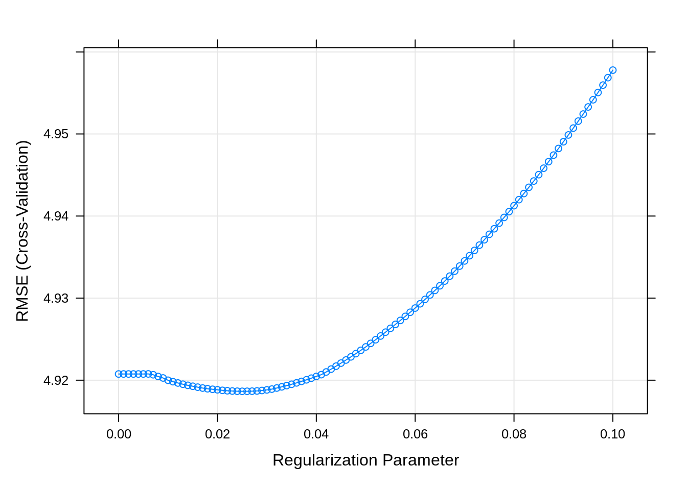
Bias-variance tradeoff

ctrl <- trainControl(method = "cv", number = 5)

# Define the tuning grid
grid <- expand.grid(alpha = 1, lambda = seq(0, 0.1, by = 0.001))

# Train the model using Lasso regression with cross-validation
lasso_fit <- train(
    medv ~ ., 
    data = df, 
    method = "glmnet", 
    trControl = ctrl, 
    tuneGrid = grid, 
    standardize = TRUE, 
    family = "gaussian"
)

plot(lasso_fit)